Table of Contents
WORKING WITH ANALYTICAL FUNCTIONS:
DEFINITION:
- Analytical functions compute an aggregate value based on a group of rows. This group of rows are called Window of rows.
- The Window determines the no of rows to be used to perform the calculation of the current row.
- Analytical function is differ from normal aggregate function as normal aggregate function returns a single row for a group of rows, while the analytical function returns multiple rows for a group of rows.
FEATURES:
- Analytical functions are the last set of operation in a query except the last order by clause.
- Joining and all other clauses like WHERE, GROUP BY, HAVING clauses are completed before the analytical functions are processed.
- Analytical functions can appear only in SELECT list or ORDER BY clause.
- Analytical functions can take 0 to 3 arguments.
- The datatype of the arguments can be any numeric data type or any data type that can be implicitly converted into numeric data types.
- The OVER analytic clause indicate that the function operates on a group of values.
- OVER clause is computed after the FROM, WHERE, GROUP BY or HAVING clauses.
- PARTITION BY clause is used to partition the query result set into multiple groups based on one or more columns provided in PARTITION BY clause.
- ORDER BY clause is used to specify how data is sorted within a partition. Multiple columns can be used in ORDER BY clause.
RESTRICTION ON ORDER BY CLAUSE:
- ASC|DESC
- NULLS FIRST|NULLS LAST
- ROW|RANGE
- BETWEEN|AND
- UNBOUNDED PRECEDING
- UNBOUNDED FOLLOWING
- CURRENT ROW
ASC|DESC:
Specify the ordering sequence as ascending or descending. Default is ASC.
NULLS FIRST|NULLS LAST:
Specify in ordering sequence whether the rows containing NULL should appear first or last.
SELECT * FROM EMPLOYEES
ORDER BY DEPARTMENT_ID NULLS FIRST;

SELECT * FROM EMPLOYEES
ORDER BY DEPARTMENT_ID NULLS LAST;

ROW|RANGE(WINDOW CLAUSE):
- ROWS specifies each row of a window which is a physical set rows and that is used for calculating the function result.
- RANGE specifies each row of a window which is a logical set rows and that is used for calculating the function result.
- These clauses cannot be used unless you have specified the ORDER BY clause.
Few example of Analytical Functions for which Window clause is applicable:
- AVG
- SUM
- COUNT
- MIN
- MAX
- FIRST_VALUE
- LAST_VALUE
- NTH_VALUE
- STDDEV
EAXMPLE 1:
SELECT EMPLOYEE_ID,
       FIRST_NAME,
       LAST_NAME,
       HIRE_DATE,
       DEPARTMENT_ID,
       SALARY,
       ROUND(SUM(SALARY) OVER(PARTITION BY DEPARTMENT_ID ORDER BY EMPLOYEE_ID ROWS 1 PRECEDING)) CUM_SUM_SAL_BW,
       ROUND(SUM(SALARY) OVER(PARTITION BY DEPARTMENT_ID ORDER BY EMPLOYEE_ID ROWS BETWEEN 0 PRECEDING AND 1 FOLLOWING)) CUM_SUM_SAL_FW,
       ROUND(SUM(SALARY) OVER(PARTITION BY DEPARTMENT_ID ORDER BY EMPLOYEE_ID ROWS BETWEEN 1 PRECEDING AND 1 FOLLOWING)) CUM_SUM_SAL_BW_FW
FROM EMPLOYEES
ORDER BY EMPLOYEE_ID;

In the first cumulative salary column CUM_SUM_SAL_BW, for department_id 90, in the 1st row since there is no previous row, its value shown same as salary column, i.e. 2640. In the second row salary value is 1870, so cumulative column 1870 is added with previous row value 2640 and total is visible as (1870 + 2640) = 4510. And in 3rd row salary value is 1870 and cumulative value is 1870 + prev. row value 1870) = 3740.

In the second cumulative salary column CUM_SUM_SAL_FW, for department_id 90, since every row added with the value of next row, in the 1st row its value shown as (2640 + 1870) = 4510. In the second row salary value is 1870, so in cumulative column 1870 is added with next row salary value 1870 and total is visible as (1870 + 1870) = 3740. And the 3rd row salary value is 1870 and since its the last row of department_id 90, cumulative value is visible as 1870.

3rd cumulative salary column CUM_SUM_SAL_BW_FW, for department_id 90, since every row added with the value of previous row as well as next row, in the 1st row its value shown as (2640 + 1870) = 4510, since there is no previous row. In the second row salary value is 1870, previous row value is 2640 & next row value is 1870, so in cumulative column total is visible as (2640 + 1870 + 1870) = 6380. In the 3rd row salary value is 1870, previous row value is 1870 and since its the last row of department_id 90, cumulative value is visible as (1870 + 1870) = 3740.
EAXMPLE 2:
SELECT EMPLOYEE_ID,
       FIRST_NAME,
       LAST_NAME,
       HIRE_DATE,
       DEPARTMENT_ID,
       SALARY,
       ROUND(AVG(SALARY) OVER(PARTITION BY DEPARTMENT_ID ORDER BY EMPLOYEE_ID ROWS BETWEEN 1 PRECEDING AND 1 FOLLOWING)) AVG_SAL
FROM EMPLOYEES
ORDER BY EMPLOYEE_ID

In the above example,
- 1st avg_sal -> for employee_id 100 and 101 avg sal = ROUND((2640 + 1870)/2) = 2255.
- 2nd avg_sal -> for employee_id 100, 101, 102 avg_sal = ROUND((2640+1870+1870)/3) = 2127………so on..
EAXMPLE 3:
SELECT EMPLOYEE_ID,
       FIRST_NAME,
       LAST_NAME,
       HIRE_DATE,
       DEPARTMENT_ID,
       SALARY,
       ROUND(AVG(SALARY) OVER(PARTITION BY DEPARTMENT_ID ORDER BY EMPLOYEE_ID ROWS BETWEEN 1 PRECEDING AND 1 FOLLOWING)) AVG_SAL,
       ROUND(SUM(SALARY) OVER(PARTITION BY DEPARTMENT_ID ORDER BY EMPLOYEE_ID ROWS BETWEEN 1 PRECEDING AND 1 FOLLOWING)) SUM_SAL,
       ROUND(MAX(SALARY) OVER(PARTITION BY DEPARTMENT_ID ORDER BY EMPLOYEE_ID ROWS BETWEEN 1 PRECEDING AND 1 FOLLOWING)) MAX_SAL,
       ROUND(MIN(SALARY) OVER(PARTITION BY DEPARTMENT_ID ORDER BY EMPLOYEE_ID ROWS BETWEEN 1 PRECEDING AND 1 FOLLOWING)) MIN_SAL,
       ROUND(FIRST_VALUE(SALARY) OVER(PARTITION BY DEPARTMENT_ID ORDER BY EMPLOYEE_ID ROWS BETWEEN 1 PRECEDING AND 1 FOLLOWING)) FIRST_SAL,
       ROUND(LAST_VALUE(SALARY) OVER(PARTITION BY DEPARTMENT_ID ORDER BY EMPLOYEE_ID ROWS BETWEEN 1 PRECEDING AND 1 FOLLOWING)) LAST_SAL
FROM EMPLOYEES
ORDER BY EMPLOYEE_ID;

All possible functions are used in above example. Impact is same like Average and Sum functions.
EXAMPLE 4:
SELECT EMPLOYEE_ID,
       FIRST_NAME,
       LAST_NAME,
       HIRE_DATE,
       DEPARTMENT_ID,
       SALARY,
       ROUND(SUM(SALARY) OVER(PARTITION BY DEPARTMENT_ID ORDER BY SALARY RANGE BETWEEN 50 PRECEDING AND 100 FOLLOWING)) CUM_SUM_SAL_LR,
       ROUND(SUM(SALARY) OVER(PARTITION BY DEPARTMENT_ID ORDER BY SALARY ROWS BETWEEN 20 PRECEDING AND 50 FOLLOWING)) CUM_SUM_SAL_SM
FROM EMPLOYEES
WHERE DEPARTMENT_ID IN (30, 50)
ORDER BY EMPLOYEE_ID;

In the above example,
- in CUM_SUM_SAL_LR column, 1st row salary value is 1210 and function is set for range between 50 and 100. So Cumulative Sum will add any value between 50 less than 1210 and any value 100 greater than 1210. Since there is no such value exists in department 30, its 1st row total is equal to the 1st row salary value 1210.
- In the 2nd row salary value is 341. There is no value exists in the range, greater than 100 of 341, but there are values in the range, 50 less than 341, i.e. (341 – 50) = 291. Such values are: 308, 319. So Cumulative total of 2nd row is (308 + 319 + 341) = 968.
- Applying the same formula in 3rd row, there is one value in the range 100 greater than 319 in department 30, i.e. 341. Also there are values in the range. 50 less than 319 i.e. (319 – 50) = 269. Such values are: 275, 286, 308, 319. So Cumulative Sum is (275 + 286 + 308 + 319 + 341) = 1529. So on…
EXAMPLE 5: (DATES)
SELECT EMPLOYEE_ID,
       FIRST_NAME,
       LAST_NAME,
       HIRE_DATE,
       DEPARTMENT_ID,
       SALARY,
       MAX(HIRE_DATE) OVER(PARTITION BY DEPARTMENT_ID ORDER BY EMPLOYEE_ID ROWS BETWEEN 1 PRECEDING AND 1 FOLLOWING) MAX_HIREDATE,
       MIN(HIRE_DATE) OVER(PARTITION BY DEPARTMENT_ID ORDER BY EMPLOYEE_ID ROWS BETWEEN 1 PRECEDING AND 1 FOLLOWING) MIN_HIREDATE,
       FIRST_VALUE(HIRE_DATE) OVER(PARTITION BY DEPARTMENT_ID ORDER BY EMPLOYEE_ID ROWS BETWEEN 1 PRECEDING AND 1 FOLLOWING) FIRST_HIREDATE,
       LAST_VALUE(HIRE_DATE) OVER(PARTITION BY DEPARTMENT_ID ORDER BY EMPLOYEE_ID ROWS BETWEEN 1 PRECEDING AND 1 FOLLOWING) LAST_HIREDATE
FROM EMPLOYEES
ORDER BY EMPLOYEE_ID;

In The above example,
- max_hiredate showing us the maximum hiredate among previous row, current row and the next row. So in the 1st row its showing the value of '21-09-05' which is the maximum of current row('17-06-03') and next row ('21-09-05').
- Similarly for 2nd row hiredate is '21-09-05', previous row hiredate is '17-06-03' and next row hiredate is '13-01-01'. So the maximum among the 3 dates is '21-09-05'..so on.
- Min_hiredate is working similar way as max_hiredate but minimum among the dates will be considered.

- First_value will be considered only the first value among the dates. In the example the first row against First_hiredate showing the value '17-06-03' which is the first value among the first row ('17-06-03') and next row ('21-09-05').
- In the second row of First_hiredate is showing the value again as '17-06-03' as this is the first value among current row ('21-09-05'), previous row ('17-06-03') and next row ('13-01-01').
- Last value will consider only the last value among the dates.
EXAMPLE 6:
SELECT EMPLOYEE_ID,
       FIRST_NAME,
       LAST_NAME,
       HIRE_DATE,
       DEPARTMENT_ID,
       SALARY,
       MAX(HIRE_DATE) OVER(PARTITION BY DEPARTMENT_ID ORDER BY HIRE_DATE RANGE BETWEEN 0 PRECEDING AND 30 FOLLOWING) MAX_HD_30_FW,
       MAX(HIRE_DATE) OVER(PARTITION BY DEPARTMENT_ID ORDER BY HIRE_DATE RANGE 30 PRECEDING) MAX_HD_30_BW,
       MAX(HIRE_DATE) OVER(PARTITION BY DEPARTMENT_ID ORDER BY HIRE_DATE RANGE BETWEEN 30 PRECEDING AND 30 FOLLOWING) MAX_HD_30_BW_30_FW,
       MAX(HIRE_DATE) OVER(PARTITION BY DEPARTMENT_ID ORDER BY HIRE_DATE RANGE BETWEEN 0 PRECEDING AND 365 FOLLOWING) MAX_HD_1YR_FW,
       MAX(HIRE_DATE) OVER(PARTITION BY DEPARTMENT_ID ORDER BY HIRE_DATE RANGE 365 PRECEDING) MAX_HD_1YR_BKW,
       MAX(HIRE_DATE) OVER(PARTITION BY DEPARTMENT_ID ORDER BY HIRE_DATE RANGE BETWEEN 365 PRECEDING AND 365 FOLLOWING) MAX_HD_1YR_BKW_1YR_FW
FROM EMPLOYEES
ORDER BY EMPLOYEE_ID;

In example 6:
- hire_date is showing the value as '17-06-03'. The The MX_HD_30_FW column showing the maximum of hire_date among all dates whose values are in the range between '17-06-03' and '17-06-03' + 30 i.e. '17-07-03'. But in hire_date column there are no such dates so that its showing '17-06-03'.
- Similarly, MAX_HD_30_BW column is showing '17-06-03' as thee is no such dates between '17-06-03'and '17-06-03' – 30 i.e. '18-05-03'. But in hire_date column there are no such dates so that its showing '17-06-03'.
- In the MAX_HD_30_BW_30_FW column the value is showing again as '17-06-03' as there are no such hire_dates range between '17-06-03' – 30 and '17-06-03' + 30.
- Same formula will be applicable for remaining fields as well.
UNBOUNDED PRECEDING:
- Its indicates that the Window starts at the first row of the partition.
- Its the start point specification and cannot be used as end point of specification.
EXAMPLE 1:
SELECT EMPLOYEE_ID,
       FIRST_NAME,
       LAST_NAME,
       HIRE_DATE,
       DEPARTMENT_ID,
       SALARY,
       MAX(HIRE_DATE) OVER(PARTITION BY DEPARTMENT_ID ORDER BY HIRE_DATE ROWS UNBOUNDED PRECEDING) MAX_HD_UB_PR,
       MIN(HIRE_DATE) OVER(PARTITION BY DEPARTMENT_ID ORDER BY HIRE_DATE ROWS UNBOUNDED PRECEDING) MIN_HD_UB_PR
FROM EMPLOYEES
WHERE DEPARTMENT_ID IN (30, 60, 90)
ORDER BY EMPLOYEE_ID;

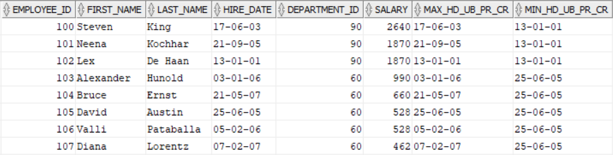
In the above example,
- The MAX_HD_UB_PR column shows the maximum of hire_date between first row and preceding rows where values is less than that of current row. In this case every row will be the maximum of all the preceding rows whose values are less than that of current row.
- The MIN_HD_UB_PR column shows the minimum of hire_dates between current row and the preceding rows whose values are less than that of current row. In this case minimum hire_date of any department will be shown against each row.
EXAMPLE 2:
SELECT EMPLOYEE_ID,
       FIRST_NAME,
       LAST_NAME,
       HIRE_DATE,
       DEPARTMENT_ID,
       SALARY,
       MAX(HIRE_DATE) OVER(PARTITION BY DEPARTMENT_ID ORDER BY HIRE_DATE ROWS BETWEEN UNBOUNDED PRECEDING AND CURRENT ROW) MAX_HD_UB_PR_CR,
       MIN(HIRE_DATE) OVER(PARTITION BY DEPARTMENT_ID ORDER BY HIRE_DATE ROWS BETWEEN UNBOUNDED PRECEDING AND CURRENT ROW) MIN_HD_UB_PR_CR
FROM EMPLOYEES
WHERE DEPARTMENT_ID IN (30, 60, 90)
ORDER BY EMPLOYEE_ID;
In case of Example 2 has the same output as Example 1 for the same reason.
EXAMPLE 3:
SELECT EMPLOYEE_ID,
       FIRST_NAME,
       LAST_NAME,
       HIRE_DATE,
       DEPARTMENT_ID,
       SALARY,
       MAX(HIRE_DATE) OVER(PARTITION BY DEPARTMENT_ID ORDER BY HIRE_DATE ROWS BETWEEN UNBOUNDED PRECEDING AND 1 FOLLOWING) MAX_HD_UB_PR_1_FO,
       MIN(HIRE_DATE) OVER(PARTITION BY DEPARTMENT_ID ORDER BY HIRE_DATE ROWS BETWEEN UNBOUNDED PRECEDING AND 1 FOLLOWING) MIN_HD_UB_PR_1_FO
FROM EMPLOYEES
WHERE DEPARTMENT_ID IN (30, 60, 90)
ORDER BY EMPLOYEE_ID;

In the Example 3,
- the current row of MAX_HD_UB_PR_1_FO will always return the next higher value within a department except its the maximum hire_date of that department. For maximum hire_date it will return the same value as the hire_date.
- In the 1st row its showing the value as '21-09-05' as in hire_date column, following next row has the value '21-09-05' and its greater than the 1st row hire_date value '17-06-03'.
- For 2nd row the hire_date and MAX_HD_UB_PR_1_FO has the same value as its the maximum value of hire_date in department 90.
- For the 3rd row the hire_date has the value '13-01-01' and next higher value in department 90 is '17-06-03', so in MAX_HD_UB_PR_1_FO column the value is showing as '17-06-03'.
EXAMPLE 4:
SELECT EMPLOYEE_ID,
       FIRST_NAME,
       LAST_NAME,
       HIRE_DATE,
       DEPARTMENT_ID,
       SALARY,
       MAX(HIRE_DATE) OVER(PARTITION BY DEPARTMENT_ID ORDER BY HIRE_DATE RANGE BETWEEN UNBOUNDED PRECEDING AND 1 FOLLOWING) MAX_HD_UB_PR_1_FO,
       MAX(HIRE_DATE) OVER(PARTITION BY DEPARTMENT_ID ORDER BY HIRE_DATE RANGE BETWEEN UNBOUNDED PRECEDING AND 1000 FOLLOWING) MAX_HD_UB_PR_1000_FO,
       MIN(HIRE_DATE) OVER(PARTITION BY DEPARTMENT_ID ORDER BY HIRE_DATE RANGE BETWEEN UNBOUNDED PRECEDING AND 1 FOLLOWING) MIN_HD_UB_PR_1_FO,
       MIN(HIRE_DATE) OVER(PARTITION BY DEPARTMENT_ID ORDER BY HIRE_DATE RANGE BETWEEN UNBOUNDED PRECEDING AND 1000 FOLLOWING) MIN_HD_UB_PR_1000_FO
FROM EMPLOYEES
WHERE DEPARTMENT_ID IN (30, 60, 90)
ORDER BY EMPLOYEE_ID;

In Example 4,
- The MAX_HD_UB_PR_1_FO column is showing the same value as that of hire_date column. Its logically searching a value one day larger than the current row.
- In First row hire_date is '17-06-03' and there is no value in department 90 where hire_date is '18-06-05'. So its showing the value as '17-06-03'. Same is repeated for 2nd and 3rd row of department 90.
- In MAX_HD_UB_PR_1000_FO column, the value is showing '21-09-05' as its logically searching a value 1000 days higher than hire_date which is '17-06-03'. So the searching range will be between '17-06-03' and ('17-06-03' + 1000) = '13-03-06'. There is only one value in department 90 in that range and i.e. '21-09-05'. In second row the hire_date and MAX_HD_UB_PR_1000_FO is showing the same value as its the maximum hire_date in department 90.
- In both MIN_HD_UB_PR_1_FO and MIN_HD_UB_PR_1000_FO the same value is showing in all rows and columns and its the minimum hire_date in department 90. With MIN function logical range will always returns the minimum in the given condition.
UNBOUNDED FOLLOWING:
SELECT EMPLOYEE_ID,
       FIRST_NAME,
       LAST_NAME,
       HIRE_DATE,
       DEPARTMENT_ID,
       SALARY,
       MAX(HIRE_DATE) OVER(PARTITION BY DEPARTMENT_ID ORDER BY HIRE_DATE ROWS BETWEEN CURRENT ROW AND UNBOUNDED FOLLOWING) MAX_HD_UB_FO,
       MIN(HIRE_DATE) OVER(PARTITION BY DEPARTMENT_ID ORDER BY HIRE_DATE ROWS BETWEEN CURRENT ROW AND UNBOUNDED FOLLOWING) MIN_HD_UB_FO
FROM EMPLOYEES
WHERE DEPARTMENT_ID IN (30, 60, 90)
ORDER BY EMPLOYEE_ID;

MORE EXAMPLES ON ANALYTICAL FUNCTION:
Query to display salary with next highest salary of employees table in descending order:
SELECT EMPLOYEE_ID,
       FIRST_NAME,
       LAST_NAME,
       EMAIL,
       HIRE_DATE,
       JOB_ID,
       SALARY,
       LEAD(SALARY, 1, 0) OVER(ORDER BY SALARY DESC) NEXT_HIGHEST_SALARY,
       (SALARY - LEAD(SALARY, 1, 0) OVER(ORDER BY SALARY DESC)) SALARY_DIFF
FROM EMPLOYEES
ORDER BY SALARY DESC;

The query to display salary with next lowest salary of employees table:
SELECT EMPLOYEE_ID,
       FIRST_NAME,
       LAST_NAME,
       EMAIL,
       HIRE_DATE,
       JOB_ID,
       SALARY,
       LAG(SALARY, 1, 0) OVER(ORDER BY SALARY) PREVIOUS_LOWEST_SALARY,
       (SALARY - LAG(SALARY, 1, 0) OVER(ORDER BY SALARY)) SALARY_DIFF
FROM EMPLOYEES
ORDER BY SALARY;

Displaying employees hire_date in ascending order with its next lowest hire_date and the gap days between two hire_dates:
SELECT EMPLOYEE_ID,
       FIRST_NAME,
       LAST_NAME, EMAIL,
       HIRE_DATE,
       LEAD(HIRE_DATE, 1, HIRE_DATE) OVER(ORDER BY HIRE_DATE) NEXT_HIRE_DATE,
       NVL((LEAD(HIRE_DATE, 1, HIRE_DATE) OVER(ORDER BY HIRE_DATE) - HIRE_DATE), 0) GAP_DAYS,
       JOB_ID,
       SALARY
FROM EMPLOYEES
ORDER BY HIRE_DATE;

Query to display employees hire_date in descending order with its previous hire_date and the gap days between two hire_dates:
SELECT EMPLOYEE_ID,
       FIRST_NAME,
       LAST_NAME, EMAIL,
       HIRE_DATE,
       LEAD(HIRE_DATE, 1, HIRE_DATE) OVER(ORDER BY HIRE_DATE DESC) PREVIOUS_HIRE_DATE,
       NVL((HIRE_DATE - LEAD(HIRE_DATE, 1, HIRE_DATE) OVER(ORDER BY HIRE_DATE DESC)), 0) GAP_DAYS,
       JOB_ID,
       SALARY
FROM EMPLOYEES
ORDER BY HIRE_DATE DESC;

RELATED TOPICS:
Nice blog here! Also your website loads up very fast! Kai Ludvig Lucine